
Forecasting ocean "weather"

Graham Rickard
Mark Hadfield
Modelling ocean currents helps focus our view of the “big picture”.
We take for granted the weather forecast: it’s a familiar feature in newspapers, radio, and television, and we spend most of our time in the atmosphere where this weather happens. We are often less aware of the effects of ocean “weather”. Though we most commonly experience only the top few metres of the sea, the coastal environment ranges to depths of many hundreds of metres and the open ocean around New Zealand plunges in places to many thousands of metres. In each of these domains there are ocean currents carrying heat and nutrients, affecting our climate, fisheries, and aquaculture. A forecast of this ocean weather would indeed be a useful thing to have.
To produce such forecasts requires good computer models for prediction, accurate observations (data) to keep the models in check, and good forecasting skill to keep the models in line. The ocean is a challenging environment to model. Ocean weather – so-called mesoscale eddying – occurs on much smaller scales than in the atmosphere, with horizontal scales of tens to hundreds of kilometers, and probing the ocean depths remains an expensive exercise. Though the ocean surface is routinely mapped from space (see “Squeezing information from an elusive ocean” in this issue), and a growing network of Argo floats collects oceanographic data (see www.argo.net), most of the ocean variability remains unmeasured.
Conversely, by building upon the measurements we do have, models can reveal the whole of the ocean. Models are mathematical representations and cannot accurately reproduce all real-world processes; for example, our present ocean model simulations don’t include the effects of tides. Nevertheless, a model is ultimately used to make a forecast, so it is relevant to try to build a model and make it perform as well as it can by comparing its output with the currently available data.
We begin with what we do know

A climatology of dynamic height (from Roemmich and Sutton). (Click these images to enlarge)

Modelled dynamic height.

Modelled transport stream function.
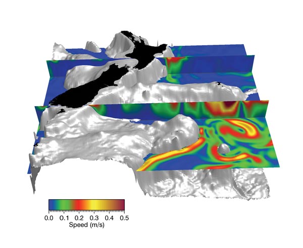
Modelled current speeds at 2000 m (horizontal slice) and on vertical slices, overlaid on the model bathymetry.
A climatology represents our best estimate of the mean state of the ocean compiled from all available data. The first image shows results from an analysis of data at NIWA. The colour shows the sea floor (bathymetry) and the contour lines show the dynamic height. Trace your finger along a contour and you will follow surface current flow; the more closely packed the contours are, the stronger that flow will be, with the circulation clockwise (cyclonic) around height minima, and anti-clockwise (anti-cyclonic) around height maxima (analogous to the isobars on a weather chart). The flow along the northeastern and eastern coasts comprises a series of quasi-permanent eddies associated with boundary currents along these coasts: the East Auckland Current flows from northwest to southeast along the top, and the East Cape Current then continues southwards.
Then compare it with a model
The next image shows the mean dynamic height according to one of the ocean models we are running at NIWA. We start the model from a resting state, and allow it to adjust over many model years in order to reach a statistically steady state. It is clear that the basic structure agrees with the climatology in the first image, particularly for the eddy off the east coast. On the other hand, compared to the climatology, the eddy structure off the northern coast is not as well defined by the model, although the East Auckland and East Cape Currents are reproduced. Note that the coastline in these figures is that represented by the model, and the coarseness reflects the fact that there is generally a compromise to be made between the time taken to run the model and the available computing power, with the result that the model has less resolution than is ideal.
Model transport streamlines shown in the image below reveal how much water is moving past a point integrated over the whole depth of the ocean. This illustrates one advantage of the model: we have access to the full three-dimensional flow field. As with the dynamic height, the contours show where all the water is moving, and the more closely packed the contours, the more material is being moved. The contour interval here is 2 Sverdrups, where a Sverdrup is one million cubic metres of ocean passing by every second (106 m3/s). It is interesting to note that these contours compare favourably with the climatological pattern in the first image, particularly in the placement of all the eddies around the coast, suggesting that the model is able to capture some of the eddy structure. These eddies are part of a highly variable western boundary current. Although the climatology represents a mean state, the actual state at any instance can vary by relatively large amounts, and is therefore a challenging region both to observe and to model.
The final image shows the model bathymetry in relief. The current flow magnitude at 2000-m depth is contoured on the horizontal slice, with vertical slices revealing currents extending down through the water column. In the foreground to the southeast is Bollons Seamount rising up some 4000 m from the sea floor, with an obvious impact on currents. Further to the west is the subantarctic slope where the New Zealand continental shelf drops steeply away. The figure shows a strong current along the slope even at 2000-m depth; this is the subantarctic front, the northernmost extent of the Antarctic Circumpolar Current (ACC) which arrives from the west, gets steered around New Zealand, then continues on its way to the east. The complex flow patterns and eddies on the 2000-m slice show that there is a strong interaction between the energetic ACC and the bathymetry. On the east coasts of both islands the vertical slices reveal significant currents: beside the South Island the Southland Current transports water northwards, and the East Cape Current flows southwards past the North Island.
Forecasting ocean weather in the future
These model runs are an attempt to reproduce the mean state, and hence understand the processes involved in shaping it. Our comparisons suggest that the models are doing a pretty good job. For an ocean forecast, however, the interest is in the state of the ocean right now.To achieve that requires data assimilation, whereby ocean observations are combined with an ocean model to obtain a best-fit picture of the ocean state, a so-called ocean analysis. In order to work towards an ocean data assimilation system, NIWA continues to assess the mean state in the models and to support critical ocean-observing programmes (such as Argo). Perhaps in the future daily weather forecasts will include conditions both above and below the sea surface.
Teachers’ resource for NCEA AS: Science 2.2; Physics 2.7; Geography 1.7, 2.7, 3.7. See other curriculum connections at www.niwa.co.nz/pubs/wa/resources